NetGraph Design and Implementation¶

NetGraph's internal design: scenario DSL, data models, execution flow, algorithms, manager components, and result handling.

Overview¶

NetGraph is a network scenario analysis engine using a hybrid Python+C++ architecture. It takes a scenario (defined in a YAML DSL) as input, builds a directed multigraph model of the network, and runs a configurable workflow of analysis steps (like traffic placement or max-flow capacity) to produce structured results.

Architecture Layers¶

Python Layer (NetGraph):

CLI and API: Entry points to load scenarios and invoke analyses
Scenario DSL Parser: Validates and expands the YAML scenario into an internal model
Domain Model: In-memory representation of nodes, links, risk groups, etc., with selection and grouping utilities
Managers: Orchestrators for higher-level behaviors (demand expansion, failure enumeration)
Workflow Engine: Composes steps into end-to-end analyses, storing outputs in a results store
Results Store: Collects outputs and metadata from each step, enabling structured JSON export
Analysis bridge: AnalysisContext builds Core graphs from the model, manages name/ID mapping, and executes Core algorithms
NetworkExplorer: Network hierarchy traversal and hardware cost/power aggregation

C++ Layer (NetGraph-Core):

StrictMultiDiGraph: Immutable directed multigraph with CSR adjacency representation
Shortest Paths (SPF): Dijkstra's algorithm with multipath support and configurable edge selection
K-Shortest Paths: Yen's algorithm for finding k-shortest simple paths
Max-Flow: Successive shortest paths with blocking flow augmentation and configurable flow placement policies
Backend Interface: Abstraction for algorithm execution (CPU backend provided)

Package Structure¶

ngraph/
├── analysis/       # AnalysisContext, FailureManager, placement
├── model/          # Network, Node, Link, demand/, failure/, flow/, selectors/
├── dsl/            # YAML parsing (blueprints/, selectors/, expansion/)
├── workflow/       # WorkflowStep implementations
├── results/        # Results store and flow result types
├── schemas/        # JSON Schema for scenario validation
├── types/          # Enums, DTOs, type aliases
├── profiling/      # Performance profiling
├── lib/            # NetworkX integration
├── utils/          # Utilities (ids, yaml, seeds)
├── scenario.py     # Scenario orchestrator
├── explorer.py     # NetworkExplorer
└── cli.py          # Command-line interface

Package Layering¶

Packages import strictly downward in this order; a lower layer never imports a higher one:

types, utils  ->  model  ->  dsl  ->  analysis  ->  workflow  ->  scenario  ->  cli

Two deliberate exceptions:

model may use the dependency-free string-expansion helpers in ngraph.dsl.expansion (bracket patterns in risk-group references and demand expand: blocks). No other model -> dsl import is allowed; selector schema types and evaluation live in ngraph.model.selectors, and ngraph.dsl.selectors re-exports them for backward compatibility. Enforced by tests/model/test_layering.py.
workflow references Scenario only under TYPE_CHECKING (workflow steps execute against a Scenario); the runtime import goes downward, from scenario to workflow.

The package root also does not eagerly import ngraph.cli (enforced by tests/cli/test_package_layering.py); the console entry point and python -m ngraph import it explicitly.

Deferred (function-local) imports are used for optional dependencies (networkx, jsonschema), opt-in profiling, and a few narrow internal cases (ngraph.model.failure.parser defers ngraph.dsl.expansion; FailureManager._process_sensitivity_results defers ngraph.results.flow) — not as a general layering workaround; outside those cases, if a module needs a lower layer, it imports it at module level.

Integration Points¶

The Python layer uses the analyze() function and AnalysisContext class (ngraph.analysis) to:

Build Core graphs from Network instances with optional pseudo-nodes for source/sink groups
Map node names (str) to NodeId (int32) and link IDs (str) to EdgeId/ext_edge_id (int64)
Execute analysis methods (max_flow, shortest_paths, sensitivity) with boolean masking
Translate results (costs, flows, paths) back to scenario-level objects

Core algorithms release the GIL, so Python threads can run them concurrently. Whether that helps depends on how much of an iteration is spent inside Core; see Failure Manager below.

Primary API:

from ngraph import analyze, Mode

# One-off analysis (unbound context)
flow = analyze(network).max_flow("^src$", "^dst$", mode=Mode.COMBINE)

# Efficient repeated analysis (bound context)
ctx = analyze(network, source="^src$", sink="^dst$", mode=Mode.COMBINE)
baseline = ctx.max_flow()
degraded = ctx.max_flow(excluded_links=failed_links)

AnalysisContext encapsulates all graph building and exposes the underlying graph components as properties for workflow steps and the FailureManager.

Execution Flow¶

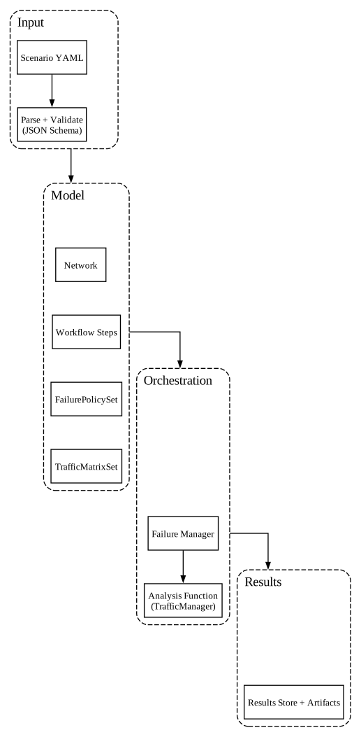
The diagram below traces a scenario from input through both layers to final results: the Python layer loads the scenario, orchestrates the workflow, and aggregates results, while compute-intensive graph algorithms execute in C++ with the GIL released.

NetGraph execution flow

Scenario DSL and Input Expansion¶

NetGraph scenarios are defined in YAML using a declarative DSL (see DSL Reference) covering network topologies, traffic demands, failure policies, and analysis workflows. Before execution, scenario files are validated against a JSON Schema, so unknown keys and type mismatches fail early.

Key elements of the DSL include:

Seed: A master random seed for the scenario to ensure deterministic behavior across runs.
Blueprints: Reusable templates for subsets of the topology. A blueprint defines internal node types, roles, and optional internal links. Blueprints enable defining a complex multi-node topology once and instantiating it multiple times with different parameters.
Node Groups: Definitions of node groups in the topology, either explicitly or via patterns. Groups can use a blueprint (blueprint) with parameters (params), or define a number of nodes (count) with a naming template (template).
Links: Rules to generate links between node groups. Instead of enumerating every link, a link rule specifies source and target selectors (by path pattern), a wiring pattern (e.g. mesh for full mesh or one_to_one for paired links), number of parallel links (count), and link properties (capacity, cost, attributes like distance, hardware, risk group tags, etc.). Link properties are specified at the top level, not inside a wrapper. Matching can also filter nodes by attributes with logical conditions (AND/OR) so a rule applies to selected nodes only. A single rule can thus expand into many concrete links.
Rules: Optional modifications applied after the initial expansion. node_rules or link_rules can match specific nodes or links (by path or endpoints) and change their attributes or disable them. This allows fine-tuning or simulating removals without changing the base definitions.
Risk Groups: Named shared-risk groups (potentially nested) that nodes or links can belong to. These are used in failure scenarios to correlate failures (e.g. all links in a risk group fail together).
Demands: Traffic demand definitions specifying source node sets, target node sets (by regex or attribute path selectors), and volume. Each demand can also include priority or custom flow placement policy.
Failure Policies: Definitions of failure scenarios or modes, possibly with weights (probabilities). For example, a policy might say "with 5% chance, fail any single core node" or "fail all links in risk_group X". The failure manager uses these policies to generate specific failure combinations for simulation.
Workflow: An ordered list of analysis steps to execute. Each step has a type (the analysis to perform, such as "MaxFlow" or "TrafficMatrixPlacement"), a unique name, and parameters (like number of iterations, etc.). The workflow definition orchestrates the analysis pipeline.

DSL Expansion Process¶

The loader validates and expands DSL definitions into concrete nodes and links. Unknown fields or schema violations cause an immediate error before any expansion. After schema validation, blueprints are resolved (each blueprint group becomes actual Node objects), group name patterns are expanded into individual names, and adjacency rules are iterated over matching source-target node sets to create Link objects. The resulting nodes and links are then checked at runtime for duplicate node names and missing link endpoints.

Data Model¶

Once the scenario is parsed and expanded, NetGraph holds it in a set of core model classes. They are the in-memory representation of the scenario topology and enforce its structural invariants: unique node names, valid link endpoints.

Node¶

A Node represents a network node (vertex). Each node has:

a unique name (string identifier),
a disabled flag (if the node is turned off in the scenario),
a set of risk_groups (associating the node with any failure domains), and
an attrs dictionary for arbitrary metadata (e.g., region, device type, hardware info)

Link¶

A Link represents a directed link between a source and target node. Each link has:

source and target node names,
capacity (float, e.g. in some bandwidth unit),
cost (float, e.g. distance or latency metric),
disabled flag,
risk_groups set,
attrs dict for metadata (e.g. distance_km, fiber type), and
a unique id assigned when the link is added to a Network

The id is deterministic: Network.add_link assigns "source|target|", where is a per-(source, target) insertion sequence number, so ids and their sort order are stable across identical scenario builds (a provisional uuid-suffixed id exists only on links never added to a Network). The model stores each link as directed (source -> target). When the analysis graph is built, a reverse edge is added by default so algorithms see bidirectional connectivity.

RiskGroup¶

A RiskGroup represents a named failure domain or shared-risk link group (SRLG). Risk groups can be hierarchical (a risk group may have children risk groups). Each RiskGroup has:

a name,
list of children RiskGroups (which inherit the failure domain property),
disabled flag (if the entire group is considered initially failed in the scenario), and
an attrs dict for any metadata

Hierarchy lets a large domain be composed of smaller sub-domains: a failure event that disables a group implicitly affects all its descendants.

Network¶

A Network is the container class that holds all nodes, links, and top-level risk groups for the scenario. The Network class maintains:

nodes: Dict[name, Node],
links: Dict[id, Link],
risk_groups: Dict[name, RiskGroup],

Network enforces invariants during construction: adding a link validates that source and target nodes exist; adding a node rejects duplicates by name. Components are never removed from the Network; the disabled flag marks them inactive. The Network also maintains a selection cache for select_node_groups_by_path to avoid repeated regex queries; cached results are copied on return (fresh dict and lists, shared Node objects), and the cache is invalidated when nodes are added.

Node and Link Selection¶

A single selector system picks groups of nodes by structured name or by attribute; algorithms use it to choose source/sink sets. Selector evaluation (schema types, condition evaluation, node selection, attribute flattening) lives in ngraph.model.selectors; ngraph.dsl.selectors provides YAML-facing parsing and re-exports the evaluation names for backward compatibility.

Selector Forms:

Selectors can be specified as:

String pattern: A regex matched against node names (anchored at start via re.match())
Selector object: A dict with path, group_by, and/or match fields

String Pattern Behavior:

When using a regex pattern, if the regex contains capturing groups, the non-None captures joined with "|" form the group label; otherwise, the entire pattern string is used as the label. For instance, the pattern r"(\w+)-(\d+)" on node name "metroA-1" produces the group label "metroA|1".

Attribute-based Grouping:

Use group_by in a selector object to group nodes by an attribute value:

source:
  group_by: "role"

This groups nodes by the value of node.attrs["role"] (e.g., "core", "leaf"), returning a dict mapping each distinct value to the list of nodes with that value. Nodes missing the attribute are excluded.

Attribute-based Filtering:

Use match in a selector object to filter nodes by attribute conditions:

source:
  path: "^dc1/.*"
  match:
    conditions:
      - attr: "tier"
        op: "=="
        value: "leaf"

Workflow steps and API calls therefore refer to nodes by readable pattern instead of by explicit list, which matters most in large topologies.

Disabled Elements¶

Nodes or links marked as disabled=True represent elements present in the design but out of service for the analysis. The base model keeps them in the collection but analysis functions filter them out when selecting active nodes. This preserves topology information — the link still exists, it is just turned off — and re-enabling it is a flag change.

Filtered Analysis (Exclusions)¶

To simulate failures or other what-if scenarios without modifying the base network, NetGraph uses analysis-time exclusions. Instead of creating a stateful view object, you pass sets of excluded nodes and links directly to analysis functions.

# Analyze with specific exclusions
results = analyze(network).max_flow(
    "^A$",
    "^B$",
    excluded_nodes={"Node5"},
    excluded_links={"A|B|xyz123"}
)

This approach avoids mutating the base graph when simulating failures (e.g., deleting nodes or toggling flags). It separates the static scenario (base network) from dynamic conditions (exclusions), enabling thread-safe parallel analyses and eliminating deep copies for each failure scenario.

Implementation: Exclusions are applied via boolean masks passed to Core algorithms. The graph is built once without exclusions, and masks disable specific elements at algorithm execution time. For repeated analysis (Monte Carlo, FailureManager) this enables O(|excluded|) mask updates rather than O(V+E) graph rebuilding. One-off calls on an unbound context build a temporary bound context per call and apply exclusions the same way.

Multiple concurrent analyses can run on the same base network with different exclusion sets, which is what makes parallel Monte Carlo over many failure combinations practical.

Graph Construction¶

NetGraph builds graphs through AnalysisContext which translates from the Python domain model to NetGraph-Core's C++ representation.

Python Side (ngraph.analysis.AnalysisContext):

There is one construction method:

AnalysisContext.from_network(): Constructs an immutable context with Core graph, mappers, algorithms instance, and pre-computed disabled topology. Bound contexts and contexts with custom augmentations build the Core graph eagerly (pseudo node IDs must be resolved at bind time); plain unbound contexts defer the Core build until first use. Exclusions are applied at algorithm call time via boolean masks rather than during graph construction.

Graph Construction Steps:

Collects nodes from Network (real + optional pseudo nodes for augmentation)
Assigns stable node IDs (sorted by name for determinism)
Encodes link_id + direction as ext_edge_id (packed int64)
Constructs NumPy arrays (src, dst, capacity, cost, ext_edge_ids)
Validates inputs: link capacities must be below the internal pseudo-edge capacity LARGE_CAPACITY (1e15), and costs must be non-negative integers whose total across all edges stays below 2^62. Core SPF accumulates path costs in int64 with INT64_MAX as the unreachable sentinel, so accumulated path costs — not just per-edge values — must stay in range; bounding the total of all edge costs bounds every path. Violations raise ValueError instead of silently corrupting results
Supports augmentation edges (e.g., pseudo-source/sink for multi-source max-flow)

AnalysisContext Internals:

AnalysisContext encapsulates pre-built graph components as internal attributes:

_handle, _multidigraph: Core graph structures
_node_mapper, _edge_mapper: Name ↔ ID translation
_algorithms: Core Algorithms instance
_disabled_node_ids, _disabled_link_ids: Pre-computed disabled topology
_link_id_to_edge_indices: Pre-computed mapping for O(|excluded|) mask building
_pseudo_context: Optional context for pseudo source/sink node mappings

When analyzing many failure scenarios, the graph is built once via AnalysisContext.from_network() and exclusions are applied via boolean masks. The public mask builders (build_node_mask/build_edge_mask, also usable by custom analysis functions that call Core primitives directly) automatically include disabled nodes/links, ensuring disabled topology is always excluded. Nothing is rebuilt per iteration, which is where the Monte Carlo speedup comes from.

Disabled Topology Handling:

Disabled nodes and links from the Network are pre-computed during AnalysisContext.from_network() and stored in the context. The mask builders automatically include these disabled elements alongside any per-iteration exclusions.

C++ Side (netgraph_core.StrictMultiDiGraph):

Immutable directed multigraph using Compressed Sparse Row (CSR) adjacency
Nodes identified by NodeId (int32), edges by EdgeId (int32)
Each edge stores capacity (float64), cost (int64), and ext_edge_id (int64)
Edges sorted by (cost, src, dst) for deterministic algorithm behavior
Zero-copy NumPy views for array access (capacities, costs, ext_edge_ids)
Neighbor iteration walks a contiguous CSR range

Edge Direction Handling:

If add_reverse=True (default), graph construction creates bidirectional edges for each network link:

Forward edge: original link direction with ext_edge_id encoding (link_id, 'fwd')
Reverse edge: opposite direction with ext_edge_id encoding (link_id, 'rev')

This allows algorithms to consider traffic flowing in both directions on physical links. The Core graph itself is always directed; bidirectionality is achieved by explicit reverse edges.

Augmentation Support:

For algorithms requiring virtual source/sink nodes (e.g., multi-source max-flow), the adapter adds augmentation edges with ext_edge_id = -1 (sentinel for non-network edges). These edges are not mapped back to scenario links in results.

Analysis Algorithms¶

NetGraph's core algorithms execute in C++ via NetGraph-Core. They operate on the immutable StrictMultiDiGraph and support masking (runtime exclusions via boolean arrays), so repeated analysis under different failure scenarios needs no graph reconstruction.

All Core algorithms release the Python GIL while they run.

Shortest-Path First (SPF) Algorithm¶

Implemented in C++ (netgraph::core::shortest_paths), using Dijkstra's algorithm with configurable edge selection and optional multipath predecessor recording.

Edge Selection Policies:

The algorithm evaluates parallel edges per neighbor using EdgeSelection configuration:

multi_edge=true (default): Include all parallel edges u→v with minimal cost among (u,v) pairs
multi_edge=false: Select single edge per (u,v) pair using tie-breaking:
PreferHigherResidual: Choose edge with highest residual capacity (secondary: lowest edge ID)
Deterministic: Choose edge with lowest edge ID for reproducibility
require_capacity=true: Only consider edges with residual capacity ≥ kMinCap (used in max-flow)
require_capacity=false (default): Consider all edges regardless of residual capacity (supplying a residual view to SPF implicitly enables the same capacity filter)

Capacity-Aware Tie-Breaking:

When multiple nodes or edges have equal cost, SPF uses residual capacity for tie-breaking to improve flow distribution:

Node-level: Priority queue ordered by (cost, -residual, node). Among equal-cost nodes, prefers paths with higher bottleneck capacity. This naturally guides flow toward higher-capacity routes.
Edge-level: When multi_edge=false and tie_break=PreferHigherResidual, selects the parallel edge with most available capacity among equal-cost options.

This tie-breaking is applied even in IP/IGP mode (require_capacity=false) using static capacities, improving flow distribution without altering routing topology.

Multipath Support:

With multipath=True, SPF stores all minimal-cost predecessors forming a DAG: pred[node] = {predecessor: [edge_ids...]}. This DAG captures all equal-cost paths in a compact form, used by max-flow for flow splitting.

Early Termination:

If dst is provided, SPF stops expanding after popping dst from the priority queue (continuing only while heap front cost equals dst cost to capture equal-cost predecessors). This optimization reduces work when only source-to-sink distances are needed.

Masking:

Optional node_mask and edge_mask boolean arrays enable runtime exclusions without rebuilding the graph. Used by FailureManager for Monte Carlo analysis.

Complexity:

Using binary heap with capacity-aware tie-breaking: (O((V+E) \log V)) time, (O(V+E)) space for costs, predecessors, and residual tracking.

Pseudocode (simplified, see implementation for complete details)¶

function SPF(graph, src, dst=None, multipath=True, edge_selection):
    costs = { src: 0 }
    pred  = { src: {} }
    min_residual_to_node = { src: infinity }  # Track bottleneck capacity for tie-breaking

    # Priority queue with node-level tie-breaking by residual capacity
    # QItem: (cost, -residual, node) - negated residual for max-heap behavior
    pq = [(0, -infinity, src)]
    best_dst_cost = None

    while pq:
        (c, neg_res, u) = heappop(pq)
        if c > costs[u]:
            continue  # stale entry

        if dst is not None and u == dst and best_dst_cost is None:
            best_dst_cost = c
        if dst is not None and u == dst:
            if not pq or pq[0][0] > best_dst_cost:
                break
            continue

        # Relax edges from u
        for v in neighbors(u):
            # Edge selection among parallel edges u->v
            min_cost = inf
            selected_edges = []

            for e_id in edges_between(u, v):
                residual_cap = residual[e_id] if has_residual else capacity[e_id]

                # Skip if capacity filtering enabled and edge has no residual
                if edge_selection.require_capacity and residual_cap < kMinCap:
                    continue

                edge_cost = cost[e_id]

                if edge_cost < min_cost:
                    min_cost = edge_cost
                    selected_edges = select_edge_by_policy(e_id, edge_selection, residual_cap)

                elif edge_cost == min_cost:
                    if edge_selection.multi_edge:
                        selected_edges.append(e_id)  # Keep all equal-cost edges
                    else:
                        # Edge-level tie-breaking for single-edge selection
                        selected_edges = tiebreak_edge(selected_edges, e_id,
                                                      edge_selection.tie_break, residual_cap)

            if not selected_edges:
                continue  # no admissible edges to v

            new_cost = c + min_cost

            # Compute bottleneck capacity: min of path residual and max edge residual
            max_edge_res = max(residual[e] for e in selected_edges)
            path_residual = min(min_residual_to_node[u], max_edge_res)

            # Relaxation: found shorter path, or (single-path mode) an
            # equal-cost path with higher bottleneck capacity
            if new_cost < costs[v] or (not multipath and new_cost == costs[v]
                                       and path_residual > min_residual_to_node[v] + epsilon):
                costs[v] = new_cost
                min_residual_to_node[v] = path_residual
                pred[v] = { u: selected_edges }
                pq.push((new_cost, -path_residual, v))  # Node-level tie-breaking by capacity

            # Multipath: found equal-cost alternative
            elif multipath and new_cost == costs[v]:
                pred[v][u] = selected_edges
                # Don't update min_residual_to_node in multipath (collecting all paths)

        if best_dst_cost is not None and (not pq or pq[0][0] > best_dst_cost):
            break

    return costs, pred


# Tie-breaking policies for edge selection when multi_edge=false:
function tiebreak_edge(current_edges, new_edge, tie_break, new_residual):
    if tie_break == PreferHigherResidual:
        # Select edge with highest residual capacity
        if new_residual > current_best_residual + epsilon:
            return [new_edge]
        elif abs(new_residual - current_best_residual) <= epsilon:
            # Secondary tie-break: deterministic by edge ID
            return [min(new_edge, current_edges[0])]
    else:  # Deterministic
        # Select edge with smallest ID for reproducibility
        return [min(new_edge, current_edges[0])]

Key Tie-Breaking Mechanisms:

Node-level tie-breaking: When multiple nodes have equal cost in the priority queue, prefer nodes reachable via paths with higher bottleneck (residual) capacity. This naturally distributes flows across equal-cost paths based on available capacity.
Edge-level tie-breaking (when multi_edge=false): - PreferHigherResidual: Among parallel equal-cost edges (u,v), select the one with highest residual capacity - Deterministic: Select edge with smallest ID for reproducible results
Multipath behavior: When multipath=true, all equal-cost predecessors are retained without capacity-based filtering, enabling flow splitting across all equal-cost paths.

Maximum Flow Algorithm¶

Implemented in C++ (netgraph::core::max_flow), using successive shortest paths with blocking flow augmentation. The algorithm blends Edmonds-Karp (augment along shortest paths) and Dinic (push blocking flows on a level graph) with cost awareness and configurable flow splitting across equal-cost parallel edges.

Goal: Compute maximum feasible flow between source and sink under edge capacity constraints.

Multi-source/multi-sink: Handled by AnalysisContext which creates pseudo-source and pseudo-sink nodes with large-capacity, zero-cost edges to/from real endpoints. The C++ algorithm operates on single source and single sink.

Routing Semantics: The algorithm's behavior is controlled by require_capacity and shortest_path:

require_capacity=true + shortest_path=false (SDN/TE): SPF filters to edges with residual capacity, routes adapt iteratively during placement
require_capacity=false + shortest_path=true (IP/IGP): SPF uses all edges based on cost, single-pass flow placement over fixed equal-cost paths

See "Routing Semantics: IP/IGP vs SDN/TE" section for detailed explanation.

The residual network is maintained via FlowState, which tracks per-edge flow and computes residual capacities on demand. For each edge u→v:

Forward residual capacity: capacity(u,v) - flow(u,v)
Reverse residual capacity: flow(u,v) (traversed to return previously placed flow during the completion phase, and for residual reachability when computing the min-cut and reachable set)

SPF operates over the residual graph by requesting edges with require_capacity=true, which filters to edges with positive residual capacity. The FlowState provides a residual capacity view without graph mutation.

Note: Reverse residual arcs are distinct from physical reverse edges added via add_reverse=True during graph construction. Physical reverse edges model bidirectional links with independent capacity; reverse residual arcs are bookkeeping over a single edge's flow. The cost-tier SPF loop traverses forward residual edges only, so it cannot cancel an earlier placement and may stop below the true maximum. A completion phase then runs BFS augmentation over the full residual graph, traversing arcs backwards to return previously placed flow, which makes the result a true maximum flow whose min-cut matches it. The completion phase applies only to max-flow semantics — PROPORTIONAL placement with require_capacity=True and shortest_path=False; EQUAL_BALANCED (ECMP admission) and require_capacity=False (fixed-cost IP routing) are placement models rather than max-flow computations and keep the tier-loop result. Dinic-style reverse edges additionally allow redistribution within a single tier's placement.

The core loop finds augmenting paths using the cost-aware SPF described above:

Run SPF from source to sink with multi_edge=true, tie_break=Deterministic, and the configured require_capacity (when true, SPF receives the residual view and filters to edges with residual capacity ≥ kMinCap). This computes shortest-path distances and a predecessor DAG over forward residual edges. The edge cost can represent distance, latency, or preference; SPF selects paths minimizing cumulative cost.

If the sink is not reached (i.e., no augmenting path exists), stop: the max flow is achieved.

Otherwise, FlowState.place_on_dag computes a blocking flow over the predecessor DAG from SPF, considering parallel edges and the splitting policy. For PROPORTIONAL: builds reversed residual graph, assigns BFS levels, uses DFS to push flow with capacity-proportional splits. For EQUAL_BALANCED: performs topological traversal with equal splits, computes global scale factor to prevent oversubscription. This yields flow amount f and per-edge flow assignments tracking which edges carry flow and their utilization.

FlowState then increases each edge's flow by its assigned portion, updating per-edge flows and residual capacities for the next iteration, and f is added to the total flow counter. If f is below tolerance kMinFlow (negligible flow placed due to numerical limits or exhausted capacity), iteration terminates; otherwise the loop repeats from the SPF step to find the next augmenting path.

If shortest_path=True, the algorithm performs only one augmentation pass and returns (useful when the goal is a single cheapest augmentation rather than maximum flow).

After the loop, the C++ algorithm computes a FlowSummary which includes:

total_flow: the sum of flow from source to sink achieved
edge_flows: per-edge flow assignments (optional, populated when requested)
residual_capacity: remaining capacity on each edge = capacity - flow (optional, populated when requested)
reachable_nodes: the set of nodes reachable from the source in the final residual network (optional, identifies the source side of the min-cut)
min_cut: the list of edges that are saturated and go from reachable to non-reachable (these form the minimum cut)
cost_distribution: flow volume keyed by cost. Tier-loop entries are the cost of the shortest-path DAG the flow was placed on; completion-phase entries are marginal costs (the augmenting path's forward edge costs minus the cost of the flow it cancels), so a key need not correspond to any traversable path. Core returns parallel arrays (costs, flows); AnalysisContext converts these to the Dict[Cost, Flow] mapping in MaxFlowResult.cost_distribution.

The summary is returned along with the total flow value.

Routing Semantics: IP/IGP vs SDN/TE¶

NetGraph models two fundamentally different routing paradigms through the require_capacity and shortest_path parameters:

IP/IGP Semantics (require_capacity=false + shortest_path=true):

Traditional IP routing with Interior Gateway Protocols (OSPF, IS-IS):

Routes computed based on link costs/metrics only, ignoring available capacity
Single SPF computation determines equal-cost paths; forwarding is fixed until topology/cost change
Traffic follows predetermined paths even as links saturate: a next hop that an earlier demand filled stays in the hash, it does not get skipped
No iterative augmentation: flow placed in single pass over fixed equal-cost DAG
Two readings of what happens when demand exceeds capacity, chosen per demand by preset: lossless admission (SHORTEST_PATHS_ECMP: how much can be carried with no drops, the planning question) or best-effort delivery (SHORTEST_PATHS_ECMP_LOSSY: how much arrives when every link carries what fits and drops the rest, the failure-impact question)
Use case: Simulating production IP networks, validating IGP designs

SDN/TE Semantics (require_capacity=true + shortest_path=false, default):

Software-Defined Networking and Traffic Engineering:

Routes adapt dynamically to residual link capacities during flow placement
SPF recomputed after each flow placement iteration, excluding saturated links
Iterative augmentation continues until max-flow achieved or capacity exhausted
Flow placement respects capacity constraints, never oversubscribing links
Models centralized traffic engineering with real-time capacity awareness
Placement is greedy and sequential: demands are placed one at a time in priority order (input order within a priority) and never revisited, so an earlier demand keeps capacity a later one would have used, and totals under contention depend on demand order. It is not a global optimum
Use case: Capacity-aware demand placement, capacity planning, failure impact analysis

This distinction is fundamental: IP networks route on cost alone with fixed forwarding tables (congestion managed via queuing/drops), while TE systems route dynamically on both cost and available capacity (congestion avoided via admission control). The require_capacity parameter controls whether SPF filters to available capacity; shortest_path controls whether routes are recomputed iteratively or fixed after initial SPF.

Flow Placement Strategies¶

Beyond routing semantics, NetGraph controls how flow splits across equal-cost parallel edges through FlowPlacement:

PROPORTIONAL (default, models WCMP/Weighted ECMP):
Splits flow across parallel equal-cost edges proportional to residual capacity
Example: Two 100G links get 50/50 split; one 100G + one 10G get 91/9 split
Maximizes utilization by preferring higher-capacity paths
Used in networks with heterogeneous link speeds (common in fabrics with multi-generation hardware)
Can be used iteratively (e.g., successive max-flow augmentations)
EQUAL_BALANCED (models traditional ECMP):
Splits flow equally across all parallel equal-cost edges regardless of capacity
Example: Two 100G links get 50/50; one 100G + one 10G still attempt 50/50 (10G saturates first)
Models IP hash-based load balancing (5-tuple hashing distributes flows uniformly)
Single-pass admission: computes one global scale factor to avoid oversubscription
The split set is every DAG edge with capacity, full or not, because a forwarding table does not react to load. A member filled by an earlier demand drives the scale to 0: any further traffic hashed onto it would be lost, so nothing more is admitted losslessly on that DAG. place_max_flow and the LSP policies progress past a full member by recomputing the DAG with a residual-aware SPF
Backs the SHORTEST_PATHS_ECMP preset; for IP ECMP simulation use require_capacity=false + shortest_path=true
EQUAL_BALANCED_LOSSY (best-effort ECMP forwarding):
Same split set, no scale: every edge carries min(share, residual) and drops the rest; a deficit propagates downstream and the placed amount is what reaches the sink
Example: one 100G + one 10G offered 100G deliver 60G and drop 40G on the 10G link
The dropped volume per edge is reported (FlowGraph.place_with_drops); backs the SHORTEST_PATHS_ECMP_LOSSY preset

FlowState.place_on_dag implements placement over a fixed SPF DAG (the DAG never changes within a call):

PROPORTIONAL: Constructs reversed residual graph from predecessor DAG. Uses Dinic-style BFS leveling and DFS push from sink to source. Within each edge group (parallel edges between node pair), splits flow proportionally to residual capacity. Distributes pushed flow back to underlying edges maintaining proportional ratios. Can be called iteratively on updated residuals.
EQUAL_BALANCED: Performs topological traversal (Kahn's algorithm) from source to sink over forward DAG. Assigns equal splits across all outgoing parallel edges from each node. Computes global scale factor as min(edge_residual / edge_assignment) across all edges to prevent oversubscription. Applies scale uniformly and stops. This models single-pass ECMP admission where the forwarding DAG doesn't change mid-flow.

Configuration Examples:

# IP/ECMP: Traditional router behavior (cost-based routing, equal splits)
analyze(network).max_flow(src, dst,
    flow_placement=FlowPlacement.EQUAL_BALANCED,
    shortest_path=True,  # Single SPF tier
    require_capacity=False)  # Ignore capacity when routing

# SDN/TE with WCMP: Capacity-aware routing with proportional splits
analyze(network).max_flow(src, dst,
    flow_placement=FlowPlacement.PROPORTIONAL,
    shortest_path=False,  # Iterative augmentation
    require_capacity=True)  # Adapt routes to capacity

# WCMP: Fixed equal-cost paths with bandwidth-weighted splits
analyze(network).max_flow(src, dst,
    flow_placement=FlowPlacement.PROPORTIONAL,
    shortest_path=True,  # Single tier of equal-cost paths
    require_capacity=False)  # Fixed paths regardless of utilization

Flow Policy Presets¶

For traffic matrix placement, FlowPolicyPreset values bundle the routing semantics above into named configurations that map to real-world network behaviors:

Preset	Behavior	Use Case
`SHORTEST_PATHS_ECMP`	IP/IGP with hash-based ECMP, lossless admission	Traditional routers (OSPF/IS-IS); `placed` is what the network carries with no drops
`SHORTEST_PATHS_ECMP_LOSSY`	IP/IGP with hash-based ECMP, best-effort delivery	Same routers under overload; `placed` is what arrives, `dropped` is lost on the way, per-link drops reported with flow details
`SHORTEST_PATHS_WCMP`	IP/IGP with weighted ECMP	Routers with WCMP support, proportional splits by residual capacity (equal to link capacity on an unloaded network)
`TE_WCMP_UNLIM`	MPLS-TE / SDN with WCMP	Capacity-aware TE with unlimited tunnels, iterative placement
`TE_ECMP_16_LSP`	MPLS-TE with 16 LSPs	Fixed 16 ECMP tunnels per demand, models RSVP-TE with LSP limits
`TE_ECMP_UP_TO_256_LSP`	MPLS-TE with up to 256 LSPs	Scalable TE with tunnel limit, models SR-TE or large-scale RSVP

Detailed Configuration Mapping (preset internals):

ngraph.model.flow.policy_config.preset_config is the single source of these values; the SPF-cached placement engine and Core's FlowPolicy both read from it.

Preset	`require_capacity`	`shortest_path`	`multi_edge`	`max_flow_count`	`flow_placement`
`SHORTEST_PATHS_ECMP`	`false`	`true`	`true`	`1`	`EQUAL_BALANCED`
`SHORTEST_PATHS_ECMP_LOSSY`	`false`	`true`	`true`	`1`	`EQUAL_BALANCED_LOSSY`
`SHORTEST_PATHS_WCMP`	`false`	`true`	`true`	`1`	`PROPORTIONAL`
`TE_WCMP_UNLIM`	`true`	`false`	`true`	unlimited	`PROPORTIONAL`
`TE_ECMP_16_LSP`	`true`	`false`	`false`	`16`	`EQUAL_BALANCED`
`TE_ECMP_UP_TO_256_LSP`	`true`	`false`	`false`	`256`	`EQUAL_BALANCED`

Key parameters (preset-managed):

require_capacity: When false, paths are selected based on link costs alone (models IP/IGP routing). When true, paths adapt to residual capacity during placement (models SDN/TE). See Routing Semantics for details.
shortest_path: When true, each demand is placed in a single pass on its cost-only shortest-path DAG and the remainder is dropped; when false, the remainder is rerouted tier by tier on residual-aware paths.
multi_edge: When true, uses all parallel equal-cost edges (hop-by-hop ECMP); when false, each flow uses a single path (tunnel/LSP semantics).
max_flow_count: Internal per-preset limit on flows/LSPs for TE presets; not a user-facing parameter.
flow_placement: EQUAL_BALANCED splits equally over the topology's next hops and admits losslessly; EQUAL_BALANCED_LOSSY splits the same way and drops what does not fit; PROPORTIONAL splits by residual capacity.

Example: Modeling IP vs MPLS Networks

# IP network with traditional ECMP (e.g., data center leaf-spine)
demands:
  dc_traffic:
    - source: ^rack1/
      target: ^rack2/
      volume: 1000.0
      flow_policy: SHORTEST_PATHS_ECMP

# MPLS-TE network with capacity-aware tunnel placement
demands:
  backbone_traffic:
    - source: ^metro1/
      target: ^metro2/
      volume: 5000.0
      flow_policy: TE_WCMP_UNLIM

Pseudocode (simplified max-flow loop)¶

function MAX_FLOW(graph, S, T, placement=PROPORTIONAL, require_capacity=True,
                  shortest_path=False):
    flow_state = FlowState(graph)  # Tracks per-edge flow and residuals
    total_flow = 0
    cost_distribution = {}  # path_cost -> flow

    while True:
        # Configure edge selection for SPF
        edge_selection = EdgeSelection(
            multi_edge=True,
            require_capacity=require_capacity,
            tie_break=Deterministic
        )

        # Find shortest augmenting paths in residual graph
        residuals = flow_state.residual_view() if require_capacity else None
        costs, dag = SPF(graph, S, T,
                        multipath=True,
                        edge_selection=edge_selection,
                        residual=residuals)

        if T not in dag:  # No augmenting path exists
            break

        # Push blocking flow through predecessor DAG
        path_cost = costs[T]
        placed = flow_state.place_on_dag(S, T, dag, infinity, placement)

        if placed < kMinFlow:  # Negligible flow placed
            break

        total_flow += placed
        cost_distribution[path_cost] += placed  # merged by exact cost

        if shortest_path:  # Single augmentation pass (IP/IGP mode)
            break

    # Completion phase: max-flow semantics only. The tier loop above walks
    # forward residual edges, so it can stop below the true maximum.
    if placement == PROPORTIONAL and require_capacity and not shortest_path:
        while True:
            # BFS over the full residual graph, including reverse arcs that
            # return previously placed flow
            path = BFS_AUGMENTING_PATH(flow_state.residual_view(), S, T)
            if path is None:
                break
            placed = flow_state.augment(path)
            if placed < kMinFlow:
                break
            total_flow += placed
            # Marginal cost: forward edge costs minus the cost of cancelled flow
            cost_distribution[marginal_cost(path)] += placed

    # Compute min-cut, reachability, cost distribution
    min_cut = flow_state.compute_min_cut(S, node_mask, edge_mask)

    return FlowSummary(
        total_flow=total_flow,
        cost_distribution=cost_distribution,
        min_cut=min_cut,
        edge_flows=...,  # optional
        residual_capacity=...,  # optional
        reachable_nodes=...  # optional
    )

The flow tolerance constant kMinFlow (1/4096 ≈ 2.4e-4) determines when flow placement is considered negligible and iteration terminates.

Each augmentation phase performs one SPF (O((V+E) \log V)) and one placement pass over the tier's predecessor DAG. For EQUAL_BALANCED the placement is a single topological pass (O(V+E)); for PROPORTIONAL it is a complete Dinic max-flow over the tier DAG (repeated BFS level construction, level-restricted blocking-flow DFS, and a group rebuild from the updated residual), worst case (O(V^2 E)). The tier loop never removes placed flow, so each phase permanently saturates at least one edge before the next SPF runs, bounding the number of phases by (O(E)); with PROPORTIONAL placement the tier's path cost also strictly increases between phases, so phases are further bounded by the number of distinct path-cost values. The resulting loose worst-case bound is (O(E \cdot (V^2 E + (V+E) \log V))). The completion phase that follows is Edmonds-Karp at (O(V E^2)), which this bound dominates.

In practice the loop stops as soon as the residual network disconnects source from sink, the number of phases equals the number of cost tiers actually used, and the kMinFlow threshold caps phases at (F / k_{MinFlow}) for total flow (F).

Managers and Workflow Orchestration¶

Managers handle scenario dynamics and prepare inputs for algorithmic steps.

Demand Expansion (ngraph.analysis.demand): Expands TrafficDemand specs (built from DSL definitions by ngraph.model.demand.builder) into concrete placement demands, resolving source/target selectors into node groups.

Deterministic expansion: node selection follows the network's stable node ordering; no randomization
Supports combine mode (aggregate via pseudo source/sink nodes attached with large-capacity, zero-cost augmentation edges) and pairwise mode (individual (src,dst) pairs, self-pairs excluded, volume split evenly across pairs)
In combine mode the pseudo source is a virtual source, a pool of the selected sources. A TE preset lets capacity decide which members originate: the aggregate is carried by whichever sources have room. Hop-by-hop presets (SHORTEST_PATHS_*) cannot steer where traffic originates, so every member that can reach a target originates an even share of the volume and routes it to its nearest targets through the pseudo sink; a member with no path to any target is not part of the split, and the result is still reported as one demand. A plain SPF from the pseudo source would keep only the sources closest to the targets, which is not a routing property of the network, so the DAG is built with Core's reverse SPF (spf_to) toward the pseudo sink with every attachment edge forced into it
Under SHORTEST_PATHS_ECMP the pool is admitted as one demand: the fan-out DAG is placed in a single equal-balanced pass, so the split ratios stay fixed and one global scale applies. A member that can carry only part of its share throttles every member alike: two equal-cost sources of capacity 100 and 10 admit 20 of a 110 demand. SHORTEST_PATHS_ECMP_LOSSY and SHORTEST_PATHS_WCMP carry each member's share independently (65 of 110 in that example); their totals and per-link drops equal those of a simultaneous pass, and shared links are attributed to members in selection order
A fixed per-source traffic matrix, where each source's share is its own and an isolated source's share is unserved rather than moved to the others, is a different question: expand per source with group_mode: per_group and group_by: name, or use pairwise
group_mode controls grouping: flatten (default, merge all groups then apply mode), per_group, and group_pairwise; volume is split evenly across groups or group pairs
In combine mode, nodes selected on both sides are excluded from the target set (prevents a zero-cost pseudo-node bypass); a demand or group whose target set empties is skipped
Validation: duplicate demand ids and pseudo-endpoint collisions raise ValueError (either would silently merge distinct demands' attachment edges)
Demands sorted by ascending priority before placement (lower value = higher priority); within a priority they keep input order, and each demand sees the residual left by the ones before it. Nothing is revisited, so contended capacity goes to the earlier demand and the totals of rerouting presets depend on demand order
Placement uses SPF caching for the hop-by-hop presets and TE_WCMP_UNLIM, FlowPolicy for the LSP presets
Non-mutating: operates on Core flow graphs with exclusions; Network remains unmodified

Failure Manager (ngraph.analysis.failure_manager): Applies a FailurePolicy to compute exclusion sets and runs analyses with those exclusions.

Parallel execution via ThreadPoolExecutor with zero-copy network sharing across worker threads; nothing is pickled, so functions defined in __main__ or notebooks can run in parallel. Threads only pay off when an iteration spends most of its time inside the core engine with the GIL released (max-flow, the LSP presets): a demand placement iteration for the hop-by-hop presets or TE_WCMP_UNLIM is mostly Python work around microsecond engine calls, and adding threads makes it slower on a GIL interpreter. TrafficMatrixPlacement therefore resolves parallelism: auto to 1 for such demand sets and to the CPU count when an LSP preset is present or the interpreter is free-threaded
Deterministic results when seed is provided (each iteration derives seed + iteration_index); with seed=None, the failure policy's own seed is used as a fallback when present
Baseline execution: a no-failure baseline is always run first as a separate reference for comparing degraded vs. intact capacity
Deduplication: identical exclusion patterns execute once and are weighted by multiplicity (occurrence_count on results; metadata["occurrence_counts"] aligned with the results list). Stored failure traces describe each pattern's representative (first) iteration; this weighting assumes deterministic analysis functions (the built-ins are)
Thread-safe analysis: Network shared by reference; exclusion sets passed per-iteration
Graph pre-building: before the iterations start, the engine calls the analysis function's prepare_inputs(network, kwargs) hook once per run and merges what it returns into every iteration's call. The built-in functions return a pre-built AnalysisContext, and demand placement also returns the expanded demands and resolved node ids. Each iteration then only builds masks, O(|excluded|). Custom analysis functions opt in by setting a prepare_inputs attribute; functions without it run with their kwargs unchanged, and passing context explicitly skips the hook.

Both the demand expansion logic and failure manager separate policy (how to expand demands or pick failures) from core algorithms. They prepare concrete inputs (expanded demands or exclusion sets) for each workflow iteration.

Workflow Engine and Steps¶

A NetGraph workflow (see Workflow Reference) is an ordered recipe of analysis steps. Each step is a pure function: it takes the current model and possibly prior results, performs an analysis, and stores its outputs. The workflow engine runs the steps in sequence and records their data in a Results store.

Common built-in steps:

BuildGraph: validates network topology and stores node-link JSON representation via NetworkX MultiDiGraph. Stores graph structure under data.graph and parameters under data.context. Primarily for validation and export; Core graph building happens in analysis functions.
NetworkStats: computes node/link counts, capacity statistics, cost statistics, and degree statistics. Supports optional excluded_nodes/excluded_links and include_disabled.
TrafficMatrixPlacement: runs Monte Carlo placement using a named demand set and the Failure Manager; a no-failure baseline always runs first. Supports iterations, parallelism, store_failure_patterns, include_flow_details, include_used_edges, and alpha or alpha_from_step (default field data.alpha_star). Produces data.baseline and data.flow_results (unique failure patterns with occurrence_count). (placement_rounds is deprecated and accepted only as a no-op for backward compatibility.)
MaxFlow: runs Monte Carlo maximum-flow analysis between node groups using the Failure Manager; a no-failure baseline always runs first. Supports mode (combine/pairwise), iterations, parallelism, shortest_path, require_capacity, flow_placement, and optional include_flow_details/include_min_cut. Produces data.baseline and data.flow_results (unique failure patterns with occurrence_count).
MaximumSupportedDemand (MSD): uses bracketing and bisection on alpha to find the maximum multiplier such that alpha * volume is feasible. Stores data.alpha_star, data.context, data.base_demands, and data.probes.
CostPower: aggregates platform and per-end optics capex/power by hierarchy level (0..N). Respects include_disabled and aggregation_level. Stores data.levels and data.context. Performs no hardware capacity/ports validation and completes even on networks the explorer's strict validation would reject; hardware validation is available via NetworkExplorer (strict validation) or the ngraph inspect command.

Each step is implemented in the ngraph.workflow module and has a corresponding type name. Steps do not modify the Network. Their inputs often include references to prior steps' results: a placement step might need the value of alpha* from an MSD step, and the workflow definition names that link.

Results storage¶

The Results object is a container that the workflow passes through steps. When a step runs, it "enters" a scope in the Results (by step name) and writes any outputs to either metadata or data within that scope.

For example, the MaxFlow step named "maxflow_between_metros" will put the total flow and details under results.steps["maxflow_between_metros"]["data"] and perhaps record parameters in metadata. The Results store also captures each step's execution metadata (like step order, type, seeds) in a workflow registry. At the end of the workflow, a single nested dictionary can be exported via Results.to_dict() containing all step outputs in a structured way.

This design ensures consistency (every step has metadata and data keys) and JSON serialization (handles custom objects via to_dict() when available, converts keys to strings). The results often include artifacts like tables or lists of flows for reporting.

Design Elements and Comparisons¶

Design choices worth knowing about:

Declarative Scenario DSL: A YAML DSL with blueprints and expansion rules turns abstract definitions (e.g., a fully meshed Clos) into concrete nodes and links. Schema validation rejects unknown or invalid fields before expansion.
Runtime Exclusions vs graph copying: Analysis-time exclusions avoid copying large structures for each scenario. The design separates static topology from dynamic failure states.
Deterministic link IDs: Network.add_link assigns each link a unique ID (source|target|<seq>, a per-endpoint-pair insertion sequence) that is stable across identical scenario builds and throughout analysis, simplifying correlation of results to original links and keeping seeded failure sampling reproducible.
Dual routing semantics: Models both IP/IGP (cost-only, fixed paths via require_capacity=false + shortest_path=true) and SDN/TE (capacity-aware, iterative via require_capacity=true + shortest_path=false)
Configurable flow placement: Proportional (WCMP-style, capacity-weighted) and Equal-Balanced (ECMP-style, uniform) splitting across parallel equal-cost edges
Cost-aware augmentation: Prefer cheapest capacity first via successive shortest paths. The cost-tier loop does not re-route previously placed flow; the max-flow completion phase may cancel earlier placements to reach the true maximum.
Deterministic simulation with seeding: Random aspects (e.g., failure sampling) are controlled by explicit seeds that propagate through steps. Runs are reproducible given the same scenario and seed.
Structured results store: Collects results with metadata in a consistent format for JSON export and downstream analysis.

Performance Considerations¶

C++ Algorithm Implementation:

Native C++ execution with optimized data structures (CSR adjacency, flat arrays)
GIL released during algorithm execution, enabling concurrent analysis across Python threads
Zero-copy NumPy integration for array inputs/outputs (via buffer protocol)
Deterministic edge ordering for reproducible results
Cache-friendly CSR representation for neighbor traversal

Graph Building and Reuse:

For Monte Carlo analysis with many failure iterations, graph construction is amortized via AnalysisContext:

Context built once before iterations begin (includes all nodes and augmentation edges)
Per-iteration exclusions applied via boolean masks rather than graph rebuilding
Mask building is O(|excluded|) using pre-computed link_id_to_edge_indices mapping
FailureManager automatically pre-builds the AnalysisContext before parallel execution (via the analysis function's prepare_inputs hook)

Graph construction involves Python processing, NumPy array creation, and C++ object initialization. Building the graph once keeps that work off the per-iteration critical path, leaving the GIL-releasing C++ algorithms to run with minimal Python overhead.

SPF Caching for Demand Placement:

Both TrafficMatrixPlacement and MaximumSupportedDemand (MSD) use a unified placement function (place_demands() in ngraph.analysis.placement) with SPF caching for cacheable policies (the SHORTEST_PATHS_* presets and TE_WCMP_UNLIM):

One SPF per unique source per mask state; later demands from the same source reuse the cached DAG. A combine-mode demand under SHORTEST_PATHS_ECMP uses one reverse SPF toward its pseudo sink instead; under the other hop-by-hop presets it is placed per source and shares each source's cache entry
For TE policies, DAG is recomputed when capacity constraints require alternate paths. Each recomputation either saturates an edge of the tier it placed on or makes no progress, so the loop is bounded by the edge count rather than by a fixed iteration cap
Complex multi-flow policies (TE_ECMP_16_LSP, TE_ECMP_UP_TO_256_LSP) use FlowPolicy directly
MSD additionally pre-resolves node IDs once at cache build time and reuses them across all alpha probes
MSD calls a scale feasible when every demand is placed to the engine's numeric resolution (a shortfall of at most 1/4096, the smallest flow the engine places) and no demand with volume placed nothing; an exact-match rule would call a demand spread over many LSPs infeasible at every scale

This reduces SPF computations from O(demands) to O(unique_sources) for workloads where many demands share the same source nodes. MSD gains the most, since it evaluates many alpha values during binary search.

Monte Carlo Deduplication:

FailureManager collapses identical failure patterns into single executions. Runtime scales with unique patterns U rather than requested iterations I; often U << I for common failure policies.